Lesson 4

Good News, but Not a Strategy Yet

Read the full distribution, sample dependence, and comparison boundaries before treating a positive event-study result as a strategy.

Hoppy stares at the result from the experiment, looking rather pleased.

“The 10-bar mean return is much higher than the result from random dates. Can we move on now?”

Dr. Hop does not answer right away.

“Do not rush to buy anything, and do not rush to add new conditions. First, let us find out what this experiment actually found.”

“Isn’t the table already clear? 1.35% is higher than 0.60%.”

“Those are the two loudest numbers in the table. They are not the whole story.”

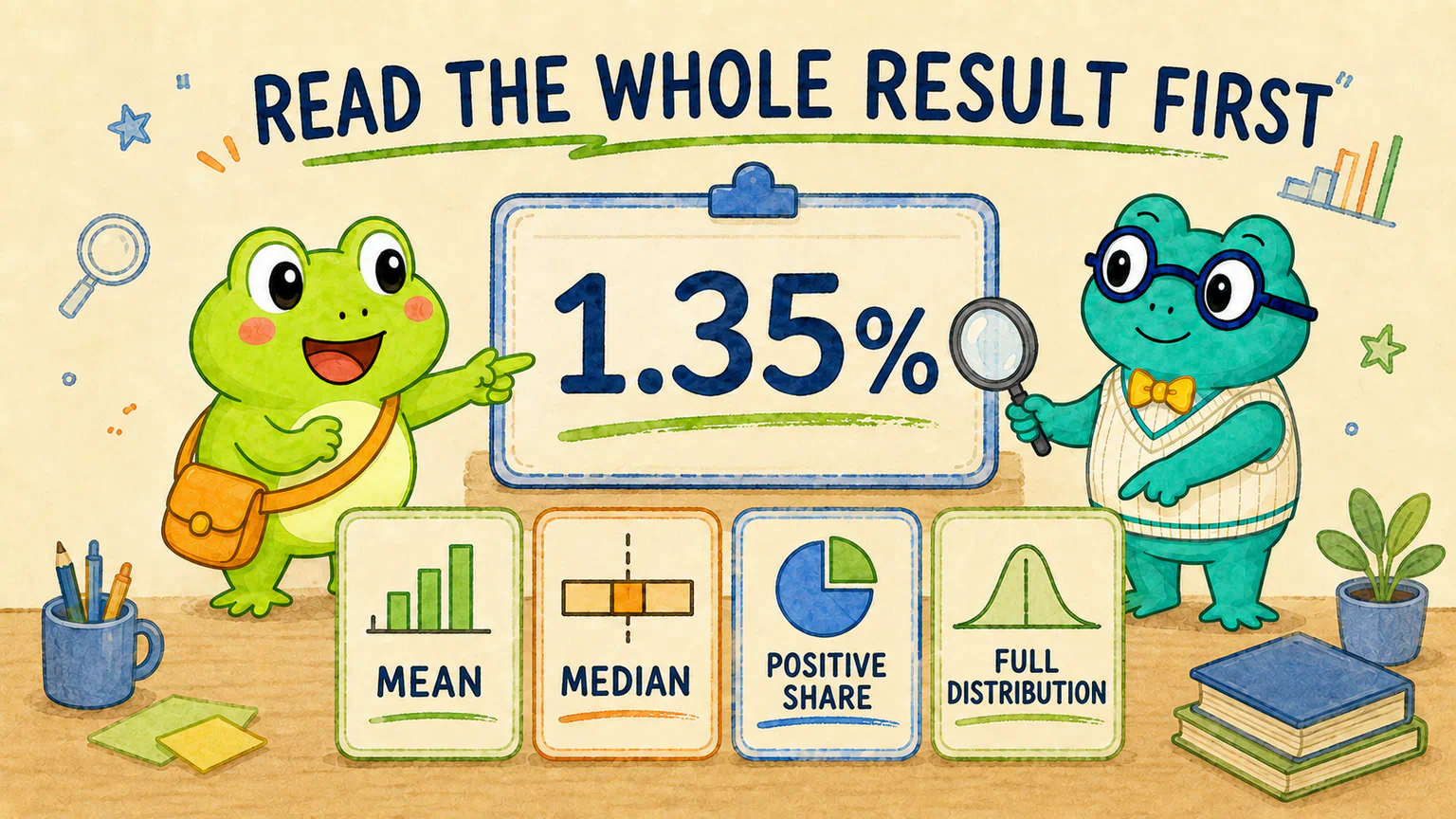
We should not read a research result by picking only its prettiest number.

The mean, median, positive-return share, and full distribution may be telling us different parts of the same story: this finding is interesting, but it is not as simple as saying, “Price rises after a nine-beat count.”

Hoppy points at the eye-catching mean return while Dr. Hop asks him to read the mean, median, positive-return share, and full distribution first. — Figure 1 | Read the mean, median, positive share, and full distribution.

Four windows, four different stories

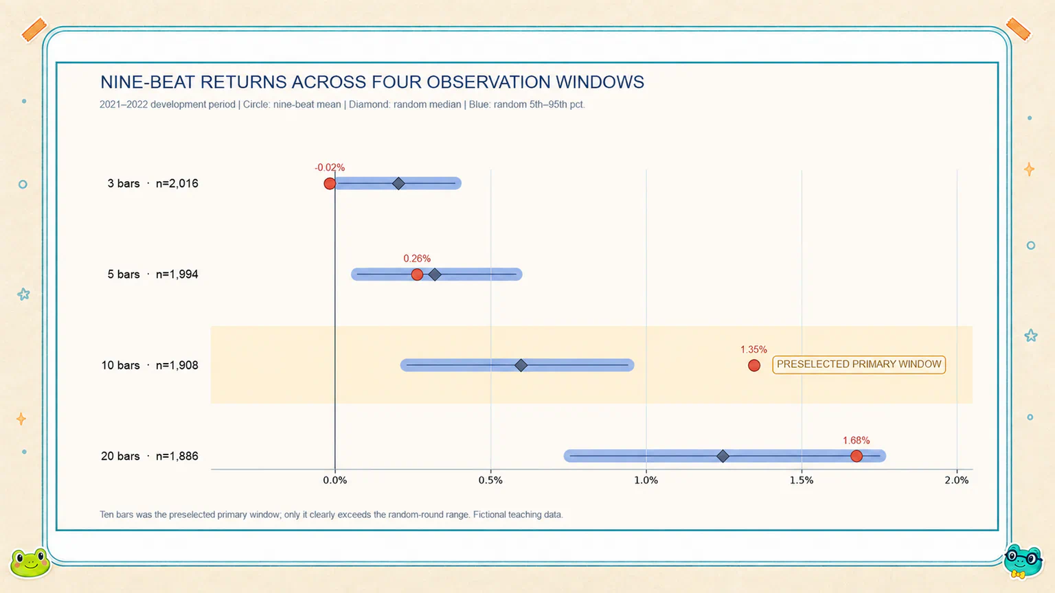
Let us put all four observation windows back on the same page:

Observation window	Mean return after a nine-beat count	Median mean return from random rounds	5th–95th percentile range of random rounds	What we see at first glance
3 bars	-0.02%	0.20%	0.01%–0.39%	Nine-beat events did slightly worse
5 bars	0.26%	0.32%	0.07%–0.58%	Very close to random dates
10 bars	1.35%	0.60%	0.23%–0.94%	The nine-beat result clearly stands out
20 bars	1.68%	1.25%	0.76%–1.75%	Higher, but random dates often reached similar results

If we look only at the nine-beat means, the 20-bar result of 1.68% is higher than the 10-bar result of 1.35%.

That does not make the 20-bar evidence stronger.

Our question is not, “Which number is largest?” It is, “Do nine-beat dates stand out from ordinary dates?”

By 20 bars, returns after random dates had risen too. The usual range of mean results from the random rounds reached as high as 1.75%, and the nine-beat result of 1.68% still sat inside that range.

In other words, drawing a batch of ordinary dates could also produce a result around that level.

The 10-bar window was different. Its nine-beat mean of 1.35% was higher than every one of the 1,000 random-round results, so it passed the weak-pattern threshold we had fixed before the experiment.

One research rule matters here: 10 bars was already our primary observation window before we saw the result.

If we shoot the arrow first and then draw the bullseye beside it, the score may look wonderful—but we have quietly changed the test.

Nine-beat mean returns and random-date ranges across four observation windows; only the preselected 10-bar window clearly exceeds the random range. — Figure 2 | The preselected 10-bar result stands out across four windows.

`1.35%` is the class average, not every event’s score

Hoppy looks at 1.35% again.

“So if I find one completed falling Nine-Beat Count, should I expect to make about 1.35% after ten bars?”

“An average height of five foot seven does not mean everyone in the room is exactly five foot seven,” Dr. Hop says. “A mean return works the same way.”

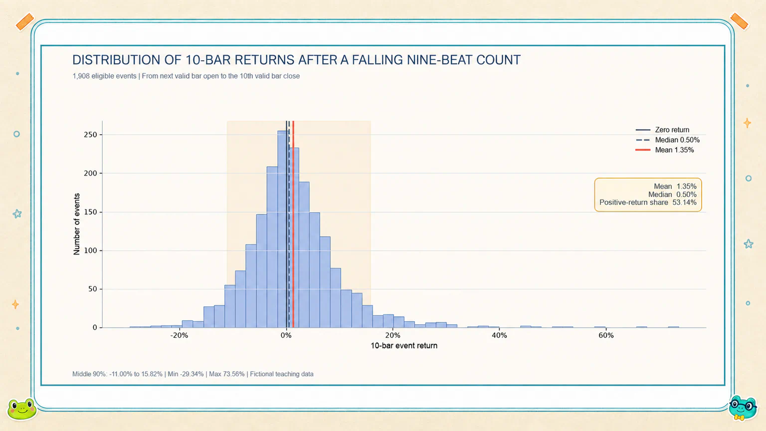
When we spread out all 1,908 eligible events, the 10-bar results look like this:

View	Result	Plain-English reading
Mean return	1.35%	Add every event return and divide by the number of events
Median return	0.50%	Put the events in order; the one in the middle returned only 0.50%
Positive-return share	53.14%	About 53 out of every 100 events had a positive return
Middle 90% range	-11.00%–15.82%	Most outcomes were widely spread, with plenty of gains and losses

This table puts the 1.35% back into its proper shape.

It does not mean “every event returned 1.35%.”

It does not even mean “almost every event made money.”

The positive-return share was only 53.14%. If we placed 100 nine-beat events in a basket, about 53 would have a positive return after ten bars, while about 47 would not.

The median was only 0.50%, noticeably below the mean. Strong events really did pull the average upward.

But the result was not held up by just one or two rockets. After removing the highest and lowest 1% of events, the mean was still 1.16%. After capping both tails at those percentile boundaries, it was 1.25%. Both checks kept the same direction.

A better description is:

After a completed falling Nine-Beat Count, 10-bar returns showed a modest upward tilt overall, but the outcomes varied greatly from one event to another.

There is a long distance between “a modest tilt” and “it rebounds every time.”

The distribution of 10-bar returns across 1,908 completed falling Nine-Beat Counts, with the mean, median, positive-return share, and middle 90% range marked. — Figure 3 | Mean, median, and distribution across 1,908 ten-bar returns.

1,908 events may still be standing in the same rainstorm

There is one more fact hiding behind the impressive count of 1,908 events.

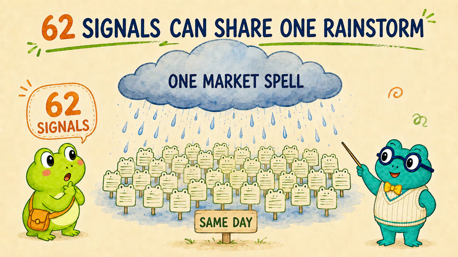
They were not spread evenly across every trading date. They appeared on only 352 completion dates, and as many as 62 falling Nine-Beat Counts completed on the same day.

For now, we care only about what that means for the evidence.

Imagine that a heavy rainstorm soaks 62 people standing on the same street.

We may record 62 wet people, but we should not treat them as 62 unrelated weather experiments. They probably met the same cloud.

Stocks can behave the same way.

Many nine-beat counts completed on the same date may share the same market environment. If the market happened to rebound, their returns might improve together. If the market kept falling, they might suffer together.

To see whether this clustering affects the conclusion, the course ran an extra check with AI after the main experiment. It grouped events that occurred on the same date or within the same stretch of market time instead of treating them as unrelated events.

This was an additional course check, not a task from the previous lesson. If your AI did not produce it, you have not missed a step. For now, focus on what it tells us.

Once we account for events sharing the same market conditions, the advantage over ordinary dates becomes less certain. We cannot rule out the possibility of no advantage.

The first experiment did meet our preset threshold. The extra check tells us not to be too confident about that advantage yet. We need to keep both findings in view.

Optional note from Dr. Hop

This check first subtracts each stock’s average return after ordinary candidate dates from each of its nine-beat event returns. A difference of zero means no return advantage; a positive difference favors the nine-beat event, and a negative difference favors ordinary dates.

It then resamples events in groups sharing a date or stretch of market time—a method called clustered resampling. Grouped by completion date, the estimated interval for that difference was -0.15%–1.57%. Grouped into consecutive 20-market-day blocks, it was -0.70%–2.21%. These intervals describe the return difference relative to ordinary dates, not the range of nine-beat returns themselves.

Both ranges crossed zero, so they did not provide the same strength of evidence as the first random-date experiment. You do not need to write a resampling program yourself. The useful idea is simple: many events do not automatically mean many fully independent pieces of evidence.

Many frogs are soaked by the same rainstorm, showing how signals on the same date may share one market environment. — Figure 4 | Same-day signals may share the same market environment.

What can we reasonably say now?

Hoppy crosses out the sentence he almost wrote—“Price rises after a nine-beat count”—and tries again:

In this study, 10-bar returns after completed falling Nine-Beat Counts stood out from returns after random dates in the same stocks. The difference appeared not only in the mean but also in the median and positive-return share. However, outcomes varied widely, and many signals were concentrated on the same market dates. For now, it is more accurate to call this a weak pattern worth investigating further.

It is not a thrilling sentence, but it is much more accurate than “A nine-beat count lets you buy the dip.”

Quantitative research is not a competition to see who can shout the boldest conclusion.

It is more like walking with a flashlight: describe what you can see, and be honest about what you cannot see yet.

If every nine-beat count is different, can we add conditions?

Once we understand the distribution, the next question appears naturally.

Taken together, all eligible falling Nine-Beat Counts showed a small historical advantage worth investigating. But their outcomes were not tidy. Some rose, some fell, some did very well, and some did very poorly.

What if we add information that was already known when each nine-beat count completed? Could that identify a group with better historical results?

For example:

What state was MACD in when the nine-beat count completed?
Was the stock’s volume high or low relative to its own usual volume?
Which market-cap group did the company belong to at that time?
Which industry did it belong to?

These conditions will not change when a nine-beat count completes, and they will not move the entry date around.

The next experiment will first keep one entry time and one temporary exit rule fixed. Then it will compare these conditions one at a time.

We do not yet know whether any of them will improve the result. One may look better, or every attempt may be worse than the unfiltered nine-beat count.

That is the question for the next experiment—not an answer we should write in advance.

Hoppy closes the result table.

The 1.35% is still there, but it no longer looks like a full stop.

It looks more like the colon before the next question.

One sentence to keep

Read the distribution and the clustering behind the average before asking how to improve it; the next research step should grow out of the evidence.

Lesson discussion

Share a question, insight, or different view—and see how other learners are thinking.